COVID-19 Number of Tests in Italy
Table of Contents
After two years, I finally decided to stop updating this page and evaluation of all code blocks has been disabled. The data was last updated on October 28/2022.
Introduction
This page presents some data about the number of tests and people tested for COVID-19 over time in Italy and compares them with the number of people found positive.
This page was created on and last updated on .
The source code available on the COVID-19 pages is distributed under the MIT License; the content is distributed under a Creative Commons - Attribution 4.0.
Getting data into R
We first read the data from the Civil Protection repository adding the ratio between positives and tests, computed on the same day and computed with data shifted by two days (on the assumption tests take two days to complete).
In fact data about tests is used with different semantics by different
regions. Some regions reports tests with results (and the ratio new
positives / tests makes sense). Other reports the number of test
performed, in which case the correct ratio is between positives and
tests performed some days earlier. We assume two days and report both
ratios for all regions. See the following issue on GitHub for an
explanation and some more details
https://github.com/pcm-dpc/COVID-19/issues/577 (in Italian).
DIGITS = 4

national = read.csv(file.path(PATH, "dpc-covid19-ita-andamento-nazionale.csv"))
national$data <- as.Date(national$data)

national$nuovi_casi_testati = c(NA, diff(national$casi_testati, 1))
national$p_over_t <- round(national$nuovi_positivi / national$nuovi_casi_testati, digits = DIGITS) * 100

national$nuovi_tamponi = c(NA, diff(national$tamponi, 1))
national$p_tamponi_over_t <- round(national$nuovi_positivi / national$nuovi_tamponi, digits = DIGITS) * 100

# national$nuovi_casi_testati_2 <- c(NA, NA, head(national$nuovi_casi_testati, -2))
# national$p_over_t_2 = round(national$nuovi_positivi / national$nuovi_casi_testati_2, digits = DIGITS) * 100

# national$nuovi_tamponi_2 <- c(NA, NA, head(national$tamponi_2, -2))
# national$p_tamponi_over_t_2 = round(national$nuovi_positivi / national$nuovi_tamponi_2, digits = DIGITS) * 100
Concerning the regional level, computed columns, such as the number of people tested in a day, have to be computed after filtering, or the diif will work on values from different regions.
# evolution over time, by Region
data = read.csv(file.path(PATH, "dpc-covid19-ita-regioni.csv"))
data$data <- as.Date(data$data)
These are the columns we are interested in and their translation in English:
cols = c(
  "data",
  "nuovi_positivi",
  "nuovi_tamponi",
  "nuovi_casi_testati",
  "p_tamponi_over_t",
  "p_over_t"
)
We now define a function to ouput the last N rows of the input data frame. The real “challenge”, here, is transposing the data, to get a more natural presentation (with time progressing from left to right).
table_data <- function(df, cols, rows = 10) {
  # get the last 10 elements and the interesting columns of the dataframe
  f  <- tail(df, rows)
  rf <- f[, cols]

  # the labels in the transposed matrix are the column names of the original data.frame
  row_labels  <- colnames(rf)
  # the columns in the trasposed matrix are the dates
  col_labels  <- c("Label", format(rf$data, "%a, %b %d"))

  rft <- data.frame(row_labels, t(rf))
  colnames(rft) <- col_labels
  return(rft[-1,])
}
People Tested and Cases in Italy
Data of the last ten days
table_data(national, cols)
| Label | Wed, Oct 19 | Thu, Oct 20 | Fri, Oct 21 | Sat, Oct 22 | Sun, Oct 23 | Mon, Oct 24 | Tue, Oct 25 | Wed, Oct 26 | Thu, Oct 27 | Fri, Oct 28 |
|---|---|---|---|---|---|---|---|---|---|---|
| nuovi_positivi | 41712 | 40563 | 36116 | 31775 | 25554 | 11606 | 48714 | 35043 | 31760 | 29040 |
| nuovi_tamponi | 233084 | 229140 | 213088 | 195575 | 161787 | 80319 | 297268 | 216735 | 205738 | 182614 |
| nuovi_casi_testati | 40696 | 40632 | 35965 | 33864 | 28465 | 15254 | 48906 | 38124 | 35350 | 33215 |
| p_tamponi_over_t | 17.9 | 17.7 | 16.95 | 16.25 | 15.79 | 14.45 | 16.39 | 16.17 | 15.44 | 15.9 |
| p_over_t | 102.5 | 99.83 | 100.42 | 93.83 | 89.77 | 76.08 | 99.61 | 91.92 | 89.84 | 87.43 |
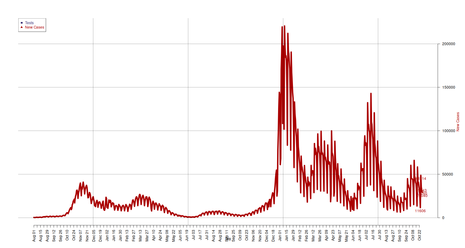
New Cases
New cases.
## add extra space to right margin of plot within frame
par(mar=c(5, 4, 4, 6) + 0.1)

## Allow a second plot on the same graph
# par(new=TRUE)
new_cases_limits = c( min(national[national$data >= "2020-08-01", c("nuovi_positivi")]), max(national[national$data >= "2020-08-01", c("nuovi_positivi")]) )

p = plot(x = national[national$data >= "2020-08-01", c("data")],
     y = national[national$data >= "2020-08-01", c("nuovi_positivi")],
     type="l", lwd=6, pch=21, cex=1.5, col=c("#AA0000"),
     axes=FALSE,
     ylim=new_cases_limits,
     ylab="", xlab="")
text(x = tail(national[national$data >= "2020-08-01", c("data")], 5),
     y = tail(national[national$data >= "2020-08-01", c("nuovi_positivi")], 5),
     labels = tail(national[national$data >= "2020-08-01", c("nuovi_positivi")], 5),
     pos = 1, cex = 1, col="#AA0000")
mtext("New Cases", side=4, line=4, col="#AA0000")
axis(4, ylim=new_cases_limits, las=1)

grid(p, col = "black", lty = "dotted")

# x-axis
dates = national[national$data >= "2020-08-01", c("data")]
axis.Date(1, at=seq(min(dates), max(dates), by="week"), format="%b %d", las=2)
mtext("Day", side=1, line=2.5)

## Add Legend
legend("topleft", legend = c("Tests", "New Cases"),
       text.col = c("#3B3176", "#AA0000"), pch= c(15, 17), col=c("#3B3176", "#AA0000"))
New Cases Tested
plot(x = national[national$data >= "2020-08-01", c("data")],
     y = national[national$data >= "2020-08-01", c("nuovi_casi_testati")],
     type="l", lwd=6, pch=16, cex=2.5, col=c("#3B3176"))
text(x = tail(national[national$data >= "2020-08-01", c("data")], 1),
     y = tail(national[national$data >= "2020-08-01", c("nuovi_casi_testati")], 1),
     labels = tail(national[national$data >= "2020-08-01", c("nuovi_casi_testati")], 1),
     pos = 4, cex = 1.2, col=c("#3B3176"))
 grid(col="black")
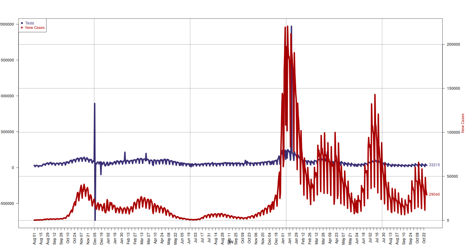
Number of Tests and New Cases Tested
Plot new cases and tests together. (Solution taken from How can I plot with 2 different y-axes? on Stack Overflow.)
## add extra space to right margin of plot within frame
par(mar=c(5, 4, 4, 6) + 0.1)

## Plot first set of data and draw its axis
tests_limits = c( min(national[national$data >= "2020-08-01", c("nuovi_casi_testati")]), max(national[national$data >= "2020-08-01", c("nuovi_casi_testati")]) )
plot(x = national[national$data >= "2020-08-01", c("data")],
     y = national[national$data >= "2020-08-01", c("nuovi_casi_testati")],
     type="l", lwd=6, pch=11, cex=1.5, col=c("#3B3176"),
     axes=FALSE,
     ylim=tests_limits,
     ylab="", xlab="")
text(x = tail(national[national$data >= "2020-08-01", c("data")], 1),
     y = tail(national[national$data >= "2020-08-01", c("nuovi_casi_testati")], 1),
     labels = tail(national[national$data >= "2020-08-01", c("nuovi_casi_testati")], 1),
     pos = 4, cex = 1, col=c("#3B3176"))
mtext("Number of Tests", side=2, col="#3B3176", line=4)
axis(2, ylim=tests_limits, col="black", las=1)
box()

## Allow a second plot on the same graph
par(new=TRUE)
new_cases_limits = c( min(national[national$data >= "2020-08-01", c("nuovi_positivi")]), max(national[national$data >= "2020-08-01", c("nuovi_positivi")]) )

p = plot(x = national[national$data >= "2020-08-01", c("data")],
     y = national[national$data >= "2020-08-01", c("nuovi_positivi")],
     type="l", lwd=6, pch=21, cex=1.5, col=c("#AA0000"),
     axes=FALSE,
     ylim=new_cases_limits,
     ylab="", xlab="")
text(x = tail(national[national$data >= "2020-08-01", c("data")], 1),
     y = tail(national[national$data >= "2020-08-01", c("nuovi_positivi")], 1),
     labels = tail(national[national$data >= "2020-08-01", c("nuovi_positivi")], 1),
     pos = 4, cex = 1, col="#AA0000")
mtext("New Cases", side=4, line=4, col="#AA0000")
axis(4, ylim=new_cases_limits, las=1)

grid(p, col = "black", lty = "dotted")

# x-axis
dates = national[national$data >= "2020-08-01", c("data")]
axis.Date(1, at=seq(min(dates), max(dates), by="week"), format="%b %d", las=2)
mtext("Day", side=1, line=2.5)

## Add Legend
legend("topleft", legend = c("Tests", "New Cases"),
       text.col = c("#3B3176", "#AA0000"), pch= c(15, 17), col=c("#3B3176", "#AA0000"))
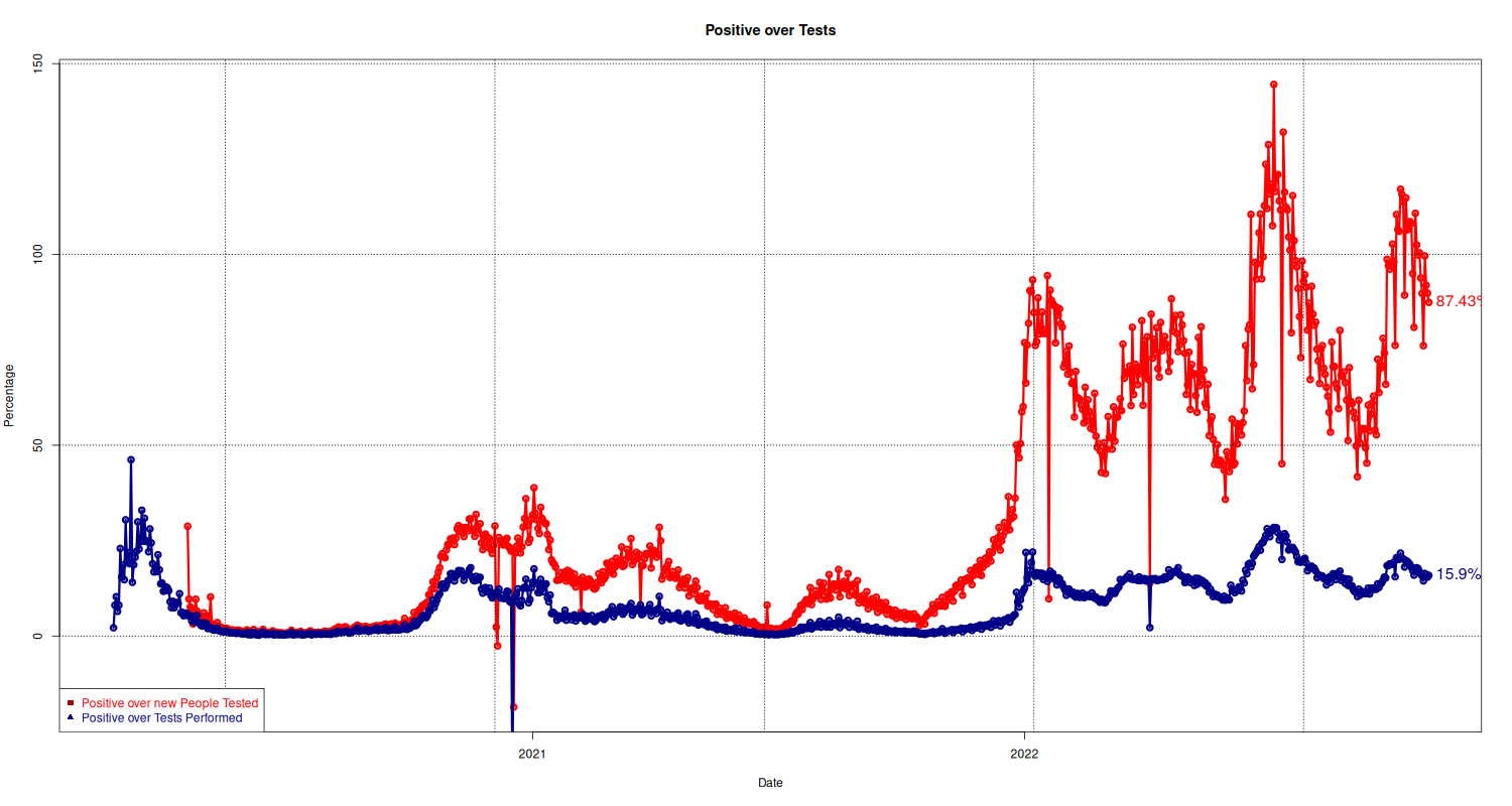
Positive/Number of Tests
Here we plot the number of positive people over tests performed. The standard measurement is the ratio between positive and tests performed (shown in blue). The way I understand it is that this number also includes tests performed on people already diagnosed and recovered.
The second graph, in red, shows the ration of positive over new people tested, that is, of all the people not yet diagnosed, how many resulted positive?
plot(national$p_over_t ~ national$data, type="o", lwd=3, pch=21, col="#ff0000", main="Positive over Tests", xlab="Date", ylab="Percentage")
text(y = tail(national, 1)$p_over_t, x = tail(national, 1)$data, lab = paste(tail(national, 1)$p_over_t, "%", sep=""), pos=4, col="#ff0000", cex=1.3)

# Second plot with Positive over tests
p = lines(national$p_tamponi_over_t ~ national$data, type="o", lwd=3, pch=21, col="#000088", xlab="Date", ylab="Percentage")
text(y = tail(national, 1)$p_tamponi_over_t, x = tail(national, 1)$data, lab = paste(tail(national, 1)$p_tamponi_over_t, "%", sep=""), pos=4, col="#000088", cex=1.3)

## Add Legend
grid(col="black")
legend("bottomleft", legend = c("Positive over new People Tested", "Positive over Tests Performed"),
       text.col = c("#ff0000", "#000088"), pch= c(15, 17), col=c("#AA0000", "#000088"))
People Tested and Cases in Trentino
region <- subset(data, denominazione_regione == "P.A. Trento")

region$nuovi_casi_testati = c(NA, diff(region$casi_testati, 1))

region$p_over_t <- round(region$nuovi_positivi / region$nuovi_casi_testati, digits = DIGITS) * 100
region$nuovi_casi_testati_2 = c(NA, NA, diff(region$casi_testati, 2))
region$p_over_t_2 = round(region$nuovi_positivi / region$nuovi_casi_testati_2, digits = DIGITS) * 100
region$nuovi_casi_testati_2 <- c(NA, NA, head(region$nuovi_casi_testati, -2))
region$p_over_t_2 = round(region$nuovi_positivi / region$nuovi_casi_testati_2, digits = DIGITS) * 100

region$nuovi_tamponi = c(NA, diff(region$tamponi, 1))
region$p_tamponi_over_t <- round(region$nuovi_positivi / region$nuovi_tamponi, digits = DIGITS) * 100
region$nuovi_tamponi_2 <- c(NA, NA, head(region$tamponi_2, -2))
region$p_tamponi_over_t_2 = round(region$nuovi_positivi / region$nuovi_tamponi_2, digits = DIGITS) * 100

table_data(region, cols)
| Label | Wed, Oct 19 | Thu, Oct 20 | Fri, Oct 21 | Sat, Oct 22 | Sun, Oct 23 | Mon, Oct 24 | Tue, Oct 25 | Wed, Oct 26 | Thu, Oct 27 | Fri, Oct 28 |
|---|---|---|---|---|---|---|---|---|---|---|
| nuovi_positivi | 578 | 545 | 477 | 400 | 314 | 119 | 485 | 386 | 301 | 269 |
| nuovi_tamponi | 2772 | 2798 | 2404 | 2197 | 1952 | 735 | 3162 | 2185 | 2065 | 1804 |
| nuovi_casi_testati | 279 | 257 | 223 | 204 | 134 | 51 | 214 | 203 | 167 | 156 |
| p_tamponi_over_t | 20.85 | 19.48 | 19.84 | 18.21 | 16.09 | 16.19 | 15.34 | 17.67 | 14.58 | 14.91 |
| p_over_t | 207.17 | 212.06 | 213.9 | 196.08 | 234.33 | 233.33 | 226.64 | 190.15 | 180.24 | 172.44 |
People Tested and Cases in Liguria
region <- subset(data, denominazione_regione == "Liguria")

region$nuovi_casi_testati = c(NA, diff(region$casi_testati, 1))

region$p_over_t <- round(region$nuovi_positivi / region$nuovi_casi_testati, digits = DIGITS) * 100
region$nuovi_casi_testati_2 = c(NA, NA, diff(region$casi_testati, 2))

region$nuovi_tamponi = c(NA, diff(region$tamponi, 1))
region$p_tamponi_over_t <- round(region$nuovi_positivi / region$nuovi_tamponi, digits = DIGITS) * 100

table_data(region, cols)
| Label | Wed, Oct 19 | Thu, Oct 20 | Fri, Oct 21 | Sat, Oct 22 | Sun, Oct 23 | Mon, Oct 24 | Tue, Oct 25 | Wed, Oct 26 | Thu, Oct 27 | Fri, Oct 28 |
|---|---|---|---|---|---|---|---|---|---|---|
| nuovi_positivi | 1113 | 1091 | 896 | 857 | 657 | 295 | 1352 | 936 | 817 | 748 |
| nuovi_tamponi | 6312 | 6161 | 5682 | 5151 | 4444 | 1984 | 8533 | 5762 | 5631 | 4918 |
| nuovi_casi_testati | 816 | 755 | 647 | 581 | 520 | 279 | 1031 | 677 | 645 | 588 |
| p_tamponi_over_t | 17.63 | 17.71 | 15.77 | 16.64 | 14.78 | 14.87 | 15.84 | 16.24 | 14.51 | 15.21 |
| p_over_t | 136.4 | 144.5 | 138.49 | 147.5 | 126.35 | 105.73 | 131.13 | 138.26 | 126.67 | 127.21 |
People Tested and Cases in Veneto
region <- subset(data, denominazione_regione == "Veneto")

region$nuovi_casi_testati = c(NA, diff(region$casi_testati, 1))
region$p_over_t <- round(region$nuovi_positivi / region$nuovi_casi_testati, digits = DIGITS) * 100

region$nuovi_tamponi = c(NA, diff(region$tamponi, 1))
region$p_tamponi_over_t <- round(region$nuovi_positivi / region$nuovi_tamponi, digits = DIGITS) * 100

table_data(region, cols)
| Label | Wed, Oct 19 | Thu, Oct 20 | Fri, Oct 21 | Sat, Oct 22 | Sun, Oct 23 | Mon, Oct 24 | Tue, Oct 25 | Wed, Oct 26 | Thu, Oct 27 | Fri, Oct 28 |
|---|---|---|---|---|---|---|---|---|---|---|
| nuovi_positivi | 5709 | 5167 | 4677 | 4486 | 3238 | 1040 | 6363 | 4772 | 4310 | 3891 |
| nuovi_tamponi | 39929 | 34525 | 32292 | 30152 | 21572 | 7816 | 48143 | 37239 | 33782 | 30803 |
| nuovi_casi_testati | 2216 | 2131 | 1706 | 1719 | 1159 | 431 | 2696 | 1913 | 1792 | 1580 |
| p_tamponi_over_t | 14.3 | 14.97 | 14.48 | 14.88 | 15.01 | 13.31 | 13.22 | 12.81 | 12.76 | 12.63 |
| p_over_t | 257.63 | 242.47 | 274.15 | 260.97 | 279.38 | 241.3 | 236.02 | 249.45 | 240.51 | 246.27 |
People Tested and Cases in Lombardia
region <- subset(data, denominazione_regione == "Lombardia")

region$nuovi_casi_testati = c(NA, diff(region$casi_testati, 1))
region$p_over_t <- round(region$nuovi_positivi / region$nuovi_casi_testati, digits = DIGITS) * 100

region$nuovi_tamponi = c(NA, diff(region$tamponi, 1))
region$p_tamponi_over_t <- round(region$nuovi_positivi / region$nuovi_tamponi, digits = DIGITS) * 100

table_data(region, cols)
| Label | Wed, Oct 19 | Thu, Oct 20 | Fri, Oct 21 | Sat, Oct 22 | Sun, Oct 23 | Mon, Oct 24 | Tue, Oct 25 | Wed, Oct 26 | Thu, Oct 27 | Fri, Oct 28 |
|---|---|---|---|---|---|---|---|---|---|---|
| nuovi_positivi | 8230 | 7983 | 6803 | 6161 | 4646 | 1640 | 9979 | 6216 | 6173 | 5504 |
| nuovi_tamponi | 43994 | 42561 | 36207 | 35098 | 30472 | 12264 | 57217 | 38317 | 36623 | 32744 |
| nuovi_casi_testati | 5011 | 4646 | 4050 | 3792 | 2894 | 1373 | 5840 | 4235 | 4033 | 3551 |
| p_tamponi_over_t | 18.71 | 18.76 | 18.79 | 17.55 | 15.25 | 13.37 | 17.44 | 16.22 | 16.86 | 16.81 |
| p_over_t | 164.24 | 171.83 | 167.98 | 162.47 | 160.54 | 119.45 | 170.87 | 146.78 | 153.06 | 155.0 |