New Cases in Italy
Table of Contents
After two years, I finally decided to stop updating this page and evaluation of all code blocks has been disabled. The data was last updated on October 28/2022.
Introduction
This page focuses on new cases in Italy. This page was created on and regularly updated since then.
R Functions
First we read the data from the CSV files of the Civil Protection repository1:
We get it into R:
# evolution over time, by Region
data = read.csv(file.path(PATH, "dpc-covid19-ita-regioni.csv"))
data$data <- as.Date(data$data)

# evolution over time at the National level
new_national = read.csv(file.path(PATH, "dpc-covid19-ita-andamento-nazionale.csv"))
new_national$data <- as.Date(new_national$data)

# latest regional data
by_region = read.csv(file.path(PATH, "dpc-covid19-ita-regioni-latest.csv"))
by_region$data <- as.Date(by_region$data)
We then output a table of new cases from R, which we then use in Ruby. (The table is not exported to HTML.)
Inferior Ruby shells perform very badly with long input lines. Make sure you
don’t pass the variable to a Ruby :session or the evaluation will break,
while IRB tries to cope with the declaration of the input variable.
If you need a :session, you should read data directly from the Ruby session,
rather than passing it as a variables.
new_national[, c("data", "nuovi_positivi")]
New Cases in Italy
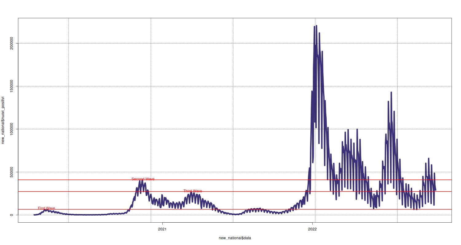
Line Plot
The shaded area corresponds to the lockdown. The red horizontal line allows to compare the latest data with historical data.
p = plot(new_national$nuovi_positivi ~ new_national$data, type="l", lwd=6, pch=16, cex=1.6, col=c("#3B3176"))
#text(new_national$nuovi_positivi ~ new_national$data, labels=new_national$nuovi_positivi, pos=2, cex=1.3)
#abline(v = as.Date("2020-10-25"), col="#FF0000", lwd=3)

grid(p, col = "black", lty="dotted")
#rect(as.Date("2020-03-09"), -200, as.Date("2020-05-19"), 7000, border = "#AA0055", col = "#AA0055", density=2)

text(x = as.Date("2020-03-25"), y = 8000, "First Wave", col="#FF0000")
abline(h = new_national[27,]$nuovi_positivi, col="#FF0000", lwd=2)
#abline(v = as.Date("2020-03-01"), col="#FF0000", lwd=2)

abline(h = 41000, col="#FF0000", lwd=2)
text(x = as.Date("2020-11-15"), y = 42000, "Second Wave", col="#FF0000")

text(x = as.Date("2021-03-16"), y = 28000, "Third Wave", col="#FF0000")
abline(h = 27354, col="#FF0000", lwd=2)
Calendar Heatmap
<<EOS
<div id="heatmap-total"></div>
<script>
calendar_heatmap.create({
    data: [
    #{data.map { |x| "{ day: \"%s\", count: %d }" % [x[0], x[1].to_i] }.join(",") }
    ],
    date_var: "day",
    fill_var: "count",
    target: "#heatmap-total"
});
</script>
EOS
New Cases by Region
Tabular Data
The table is built as follows:
egrepselects entries in the current month, getting the current month from thedatecommand- the first
sedgets rid of the “T17:00:00” timestamp in dates - the second
sedcompacts the date, by removing the year and replacing the month number with its name datamashpivots the table by region and date
current_month=$(date +"%b")
current_month_no=$(date +"%m")
year=$(date +"%Y")

egrep ${year}-${current_month_no} ./data/dpc-covid19-ita-regioni.csv | sed -e "s/T1[78]:00:00//g" | sed -e "s/${year}-${current_month_no}-/${current_month} /g" | datamash -t, crosstab 4,1 sum 13
| Oct 01 | Oct 02 | Oct 03 | Oct 04 | Oct 05 | Oct 06 | Oct 07 | Oct 08 | Oct 09 | Oct 10 | Oct 11 | Oct 12 | Oct 13 | Oct 14 | Oct 15 | Oct 16 | Oct 17 | Oct 18 | Oct 19 | Oct 20 | Oct 21 | Oct 22 | Oct 23 | Oct 24 | Oct 25 | Oct 26 | Oct 27 | Oct 28 | |
| Abruzzo | 1036 | 861 | 472 | 1889 | 1279 | 1190 | 1053 | 1200 | 895 | 427 | 1683 | 1189 | 1148 | 1035 | 892 | 702 | 424 | 1332 | 1080 | 1004 | 842 | 789 | 634 | 337 | 1230 | 915 | 821 | 767 |
| Basilicata | 229 | 165 | 134 | 298 | 193 | 162 | 184 | 173 | 165 | 117 | 281 | 192 | 217 | 180 | 183 | 132 | 107 | 261 | 134 | 165 | 122 | 141 | 109 | 87 | 230 | 142 | 141 | 159 |
| Calabria | 775 | 601 | 368 | 1390 | 838 | 898 | 933 | 861 | 737 | 430 | 1384 | 842 | 981 | 857 | 764 | 577 | 326 | 1261 | 830 | 791 | 722 | 703 | 528 | 283 | 1018 | 691 | 688 | 619 |
| Campania | 2035 | 1846 | 768 | 3377 | 2178 | 2281 | 2173 | 2325 | 1935 | 991 | 3839 | 2487 | 2401 | 1891 | 2193 | 1764 | 782 | 3473 | 2246 | 2336 | 2078 | 1951 | 1592 | 812 | 2992 | 2009 | 1918 | 1763 |
| Emilia-Romagna | 2876 | 2758 | 1964 | 2721 | 4508 | 3897 | 4095 | 4005 | 3794 | 2194 | 3258 | 4853 | 4070 | 3719 | 3335 | 3276 | 2024 | 2786 | 4133 | 3573 | 3296 | 2944 | 2586 | 1705 | 2151 | 3384 | 2961 | 2660 |
| Friuli Venezia Giulia | 1254 | 752 | 336 | 1986 | 1689 | 1415 | 1401 | 1471 | 833 | 425 | 1947 | 1509 | 1435 | 1139 | 1302 | 740 | 308 | 1599 | 1371 | 1173 | 926 | 941 | 568 | 291 | 1408 | 1010 | 947 | 760 |
| Lazio | 2810 | 2708 | 1437 | 4722 | 3474 | 3771 | 3430 | 3475 | 3023 | 1781 | 5245 | 3670 | 3875 | 3233 | 3289 | 2738 | 1637 | 4710 | 3533 | 3657 | 3316 | 2903 | 2674 | 1535 | 4644 | 3279 | 2981 | 2900 |
| Liguria | 882 | 706 | 358 | 1590 | 1163 | 1155 | 1093 | 1130 | 903 | 379 | 1853 | 1228 | 1182 | 1096 | 1115 | 771 | 328 | 1737 | 1113 | 1091 | 896 | 857 | 657 | 295 | 1352 | 936 | 817 | 748 |
| Lombardia | 5991 | 4896 | 1847 | 12249 | 8498 | 9124 | 8699 | 8671 | 6231 | 2229 | 14025 | 9126 | 8771 | 7991 | 7701 | 5653 | 1864 | 12757 | 8230 | 7983 | 6803 | 6161 | 4646 | 1640 | 9979 | 6216 | 6173 | 5504 |
| Marche | 1026 | 999 | 447 | 1864 | 1188 | 1353 | 1384 | 1134 | 989 | 501 | 2067 | 1294 | 1335 | 1239 | 1120 | 1044 | 409 | 1533 | 1058 | 1020 | 973 | 842 | 689 | 317 | 1358 | 844 | 858 | 737 |
| Molise | 123 | 137 | 102 | 133 | 164 | 142 | 139 | 107 | 140 | 80 | 167 | 161 | 146 | 143 | 143 | 145 | 47 | 138 | 147 | 122 | 138 | 91 | 93 | 50 | 123 | 90 | 94 | 105 |
| P.A. Bolzano | 570 | 362 | 187 | 1305 | 758 | 843 | 788 | 754 | 470 | 221 | 1399 | 832 | 852 | 807 | 706 | 385 | 198 | 1159 | 641 | 623 | 470 | 478 | 218 | 124 | 683 | 404 | 358 | 291 |
| P.A. Trento | 639 | 512 | 159 | 1013 | 760 | 804 | 744 | 726 | 585 | 144 | 1142 | 881 | 749 | 638 | 636 | 446 | 127 | 789 | 578 | 545 | 477 | 400 | 314 | 119 | 485 | 386 | 301 | 269 |
| Piemonte | 3249 | 2754 | 1341 | 7547 | 4899 | 4659 | 5010 | 4874 | 3672 | 1335 | 7812 | 5170 | 4991 | 4240 | 3843 | 2865 | 1480 | 6818 | 3946 | 4341 | 4305 | 2068 | 2181 | 829 | 4822 | 3102 | 2115 | 1999 |
| Puglia | 1271 | 954 | 442 | 2067 | 1343 | 1365 | 1339 | 1408 | 1122 | 510 | 2366 | 1644 | 1601 | 1441 | 1486 | 1137 | 464 | 2331 | 1469 | 1464 | 1352 | 1294 | 1018 | 417 | 2104 | 1319 | 1327 | 1209 |
| Sardegna | 352 | 246 | 224 | 922 | 631 | 723 | 650 | 497 | 416 | 383 | 1215 | 750 | 751 | 756 | 565 | 471 | 325 | 1200 | 740 | 757 | 568 | 620 | 485 | 235 | 1114 | 703 | 657 | 618 |
| Sicilia | 1188 | 1058 | 498 | 1873 | 1430 | 1270 | 1403 | 1221 | 1090 | 532 | 1854 | 1595 | 1443 | 1383 | 1257 | 1169 | 535 | 2071 | 1608 | 1520 | 1408 | 1282 | 1281 | 542 | 2127 | 1562 | 1331 | 1472 |
| Toscana | 1883 | 1514 | 524 | 3637 | 2504 | 2649 | 2345 | 2547 | 1809 | 581 | 4085 | 2716 | 2675 | 2373 | 2341 | 1664 | 512 | 3459 | 2213 | 2282 | 1890 | 2044 | 1361 | 612 | 3485 | 2381 | 2192 | 1918 |
| Umbria | 806 | 776 | 451 | 1198 | 1078 | 1143 | 984 | 963 | 888 | 416 | 1202 | 1072 | 1023 | 883 | 887 | 734 | 304 | 1015 | 812 | 828 | 764 | 705 | 627 | 306 | 923 | 816 | 679 | 600 |
| Valle d’Aosta | 77 | 58 | 42 | 182 | 141 | 128 | 175 | 101 | 89 | 35 | 228 | 142 | 120 | 121 | 107 | 75 | 29 | 187 | 121 | 121 | 93 | 75 | 55 | 30 | 123 | 82 | 91 | 51 |
| Veneto | 4804 | 3846 | 1215 | 8312 | 6509 | 5881 | 6650 | 6073 | 4658 | 1378 | 8873 | 6410 | 5939 | 5415 | 5104 | 3751 | 1209 | 7744 | 5709 | 5167 | 4677 | 4486 | 3238 | 1040 | 6363 | 4772 | 4310 | 3891 |
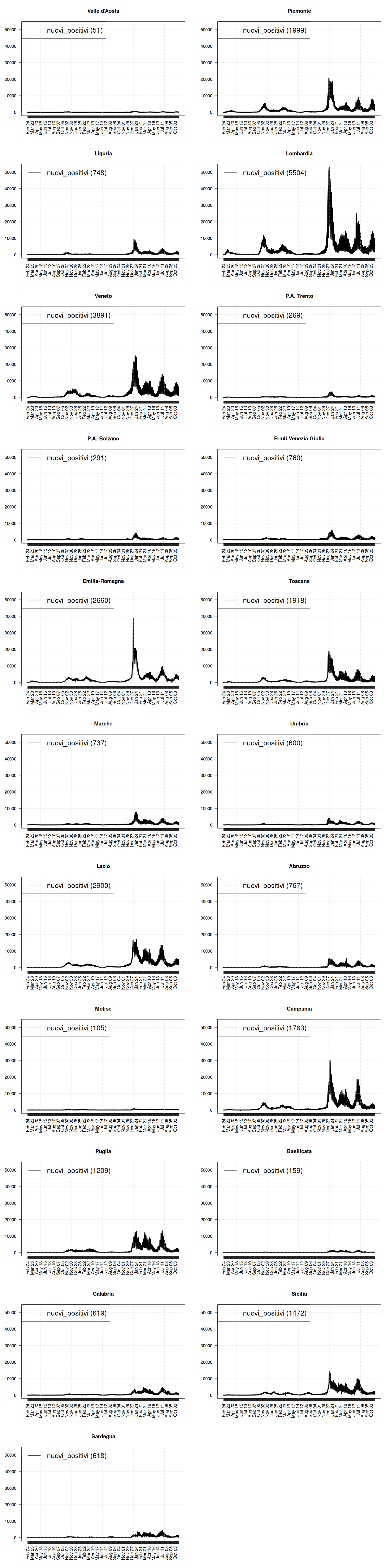
Line Plots
# how many rows and columns?
par(mfrow=c(11, 2))
regions <- c("Valle d'Aosta", "Piemonte", "Liguria", "Lombardia", "Veneto",
             "P.A. Trento", "P.A. Bolzano", "Friuli Venezia Giulia",
             "Emilia-Romagna", "Toscana", "Marche", "Umbria",
             "Lazio", "Abruzzo", "Molise", "Campania",
             "Puglia", "Basilicata", "Calabria", "Sicilia",
             "Sardegna")
for (region in regions) {
  my_plot(region,
          data,
          max=max(data$nuovi_positivi),
          filter=TRUE,
          textlabels=FALSE,
          variables=c("nuovi_positivi"),
          graphtypes=c("l"),
          colors=c("black"))
}
The source code available on the COVID-19 pages is distributed under the MIT License; the content is distributed under a Creative Commons - Attribution 4.0.
Footnotes:
The CSV files containing the data are updated by the first code block in index.html.